You don't have to be an Excel spreadsheet whiz to create your own amortization table. All the formulas have been pre-calculated for you, so you need only to key them into the appropriate cells. Just follow these simple step-by-step instructions to build your table in a matter of minutes, or alternatively you can use a free amortization calculator.
Excel Amortization Table Instructions
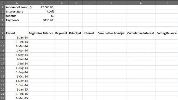
As an example, assume this is a five-year (60 month) loan, for $22,000, at an interest rate of 7 percent. Once you get the basics in place, you can customize the table to reflect any loan terms you wish.
- Open a new Excel spreadsheet.
- Starting with A1, list these categories in column A:
- Amount of Loan
- Interest Rate
- Months
- Payments
- Starting with B1, assign values for the first three categories in column B:
- $22,000
- 7% (Note: The interest rate must be entered as a percentage.)
- 60
- In B4 enter the following formula and click "enter": =PMT($B$2/12,$B$3,-$B$1,0)
- List the following categories in row 7, beginning with A7:
- Period
- Beginning Balance
- Payment
- Interest
- Cumulative Principle
- Cumulative Interest
- Ending Balance
- In cell A8 key in the date the first payment is due, and press "enter."
- Select A8 and, using the cell's bottom right handle, drag it down through A67, highlighting each cell.
- Make sure the auto fill option is set to "Months."
- To access the settings, click the pull down menu that appears to the bottom right of the final cell selected.
- Make sure the auto fill option is set to "Months."
- At this point your spreadsheet should look like this:
- In cell B8 enter the beginning balance of the loan, in this example, $22,000
- In cell C8 enter the following formula and press "enter": =$B$4
- In cell E8 enter the following formula and press "enter": =$B8*($B$2/12)
- In cell D8 enter the following formula and press "enter": =$C8-$E8
- In cell H8 enter the following formula and press "enter": =$B8-$D8
- In cell B9 enter the following formula and press "enter": =$H8
- Copy cells C8, D8 and E8 and paste them into C9, D9 and E9
- Copy cell H8 and paste it into H9
- In cell F9 enter the following formula and press "enter": =$D9+$F8
- In cell G9 enter the following formula and press "enter": =$E9+$G8
- Ensure that cells A8 through H8 and A9 through are formatted for currency
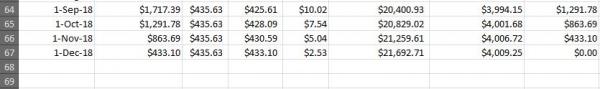
- Select cells B9 through H9 and drag down to populate the remainder of your amortization table
- The last cell in column H (in this example, H67) should end in $0.00. If it does not, recheck the formulas entered.
- The last few rows of your table should look like this:
- To protect the ongoing accuracy of your table, lock all the cells that contain formulas.
- Select all the cells you want to lock and click the "Format" icon at the top of the Excel spreadsheet.
- Click "Lock Cell"
Customizing the Table
Now that the basic amortization table has been created, you can customize it to calculate nearly countless loan scenarios. For example, if you want to amortize a 30 year (360 months) mortgage you will need 360 rows for payment information.
- Refer back to Step 8. Instead of dragging your cursor through 60 cells (stopping at A67), you will need to drag it through 360 cells (stopping at A367).
- Key the amount of the loan into cell B1 and press "enter."
- Key the annual interest rate into cell B2 and press "enter."
- Key the number of months that payments will be due into B3, and press "enter."
Congratulations! Your brand-new loan scenario just auto-calculated for you.
Using Amortization Tables
Amortization tables allow you to experiment with a variety of loan variables. With a few clicks you can easily determine the overall amount of interest you would pay on a 15-year mortgage, versus a 30-year, or what would be the impact of a one percent interest change to your monthly payment. These types of calculations often yield surprising insights and provide you with the information you need to make good decisions.